The number of ways you can use Excel is countless, and so are the number of features packed inside Microsoft’s most popular number-crunching application. Whether you’re a casual user or an Excel expert, it pays to know everything that the program’s capable of, and here are 18 easy tricks that can make a difference.

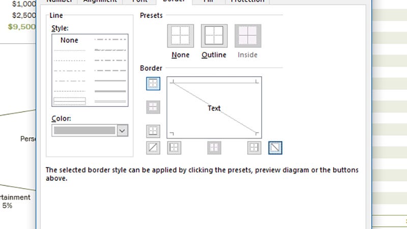
1) Apply diagonal borders

If you’ve got a table that needs labels for both the row and column headers in the same cell, use diagonal borders. Click More Borders at the bottom of the borders drop-down menu (on the Home tab of the ribbon), and the diagonal buttons are by the box corners.

2) Insert multiple rows and columns

You probably know you can select a row or column then add a new one via the Insert drop-down under Home. What you might not be aware of is if you select multiple rows or columns to begin with (like 5 or 10), then Excel adds in that many extra gaps in your sheet.

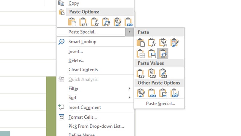
3) Turn columns into rows (or vice versa)

If you have data in columns that should be in rows or the other way around (whether through your own fault or someone else’s), all is not lost. Copy the original block of cells, then right-click on the destination cell, and choose Paste Special then Transpose.

4) Hide individual cells

Excel has a trick for ‘hiding’ cells. With the cells selected, right-click, choose Format Cells and then set the format as Custom under the Number tab. Enter ;;; (three semicolons) as the format. The cell contents disappear but they’re still there and can be used in formulas.

5) Save time with Flash Fill

If you’re reformatting data (like the names above) in an adjacent column, Flash Fill will recognize patterns and fill out the rest of the details for you. Just give Excel a few examples at the top. You should see suggestions in gray, so hit Enter to accept.

6) Freeze row and column headings

One of the simplest and oldest Excel tricks is to freeze row and column headings so they’re always in view while you scroll around. Place the cursor in the top-left cell where the actual data starts, then choose Freeze Panes and Freeze Panes from the View menu.

7) Add comments to your formulas

Add a space then

+N(“your
comment here”)

to leave comments by your formulas, either for your own reference or to help other people understand your spreadsheet. Comments don’t appear in the cell but do show up in the Formula bar, and they’re searchable too.

8) Quickly add up figures

It’s likely that you’re going to be doing a lot of addition with Excel, but you don’t have to type out SUM formulas. Highlight the cell at the end of the row or the bottom of the column you want to add up, then hit Alt+= (equals) or Cmd+Shift+T on a Mac.

9) Rotate heading text

If you need to add headers to very narrow columns, you can rotate the text to fit. The button you need is labelled Orientation and is on the Home tab alongside the other text formatting options. With the right cells selected, click it once and make your choice.

10) Add decimal points automatically

You don’t have to waste time manually inserting decimal points because Excel can do it for you: click File, Options, Advanced and the option is near the top. There are various other handy settings on this page too, covering program behavior, number formats and more.

11) Add your own graphics to charts

You don’t have to settle for the colored blocks that Excel gives you by default when it comes to creating charts. Double-click on a bar, then click the paint bucket to change the fill options: you can switch to a gradient, a pattern, or load in an image file from disk.

12) Save your charts as templates

Here’s another handy chart-related trick. When you’ve found a combination of layout and colors that you’re really keen on, save it as a template so you can use it again. Simply right-click on any chart you’ve created and you’ll see the Save as Template option.

13) Add the Calculator (or something else) to Quick Access

Open up the Quick Access Toolbar (to the right of the save and undo commands on the title bar), choose More Commands, and you can add a Calculator shortcut to the menu, or something else, like a shortcut to the Windows Camera or Ink apps, or the zoom controls.

14) Select everything at once

A useful shortcut you might not yet have discovered. That little box where the row headings and column headings meet can be used to select the entire sheet, if you click on it. Alternatively, just press Ctrl+A (or Cmd+A) on your keyboard for the same end result.

15) Apply some conditional formatting

Conditional formatting can add some pop to your sheets and help you pick out data easily, and it’s simple to use. Select the data to be formatted, click Conditional Formatting (under Home), then build your rules accordingly from the drop-down options.

16) Quickly resize columns and rows

You can resize columns and rows by right-clicking or by dragging the row or heading boundaries at the edges of your sheets with the mouse. There’s a quicker option, though. Double-click a row or column heading border to automatically resize it to fit the data.

17) Draw out equations

If you find it easier to draw out equations, this is now possible in Excel 2016 (handy if you’ve got a touchscreen computer too). Go to the Insert tab on the ribbon menu, then choose Equation and Ink Equation. You can then sketch away in the yellow box.

18) Learn Excel’s best shortcut keys

If you really want to improve your productivity on Excel, learn some shortcut keys to do common tasks faster. There are lots of them to pick from, including Ctrl+; to insert today’s date, F2 to edit the current cell, and Alt+Enter to start a new line in the cell you’re in.

The Creative Apprentice

Thursday, September 13, 2018

18 Tricks to Make Yourself a Microsoft Excel Master